Venkatesh Ravichandran

Understanding Stochastic Gradient Descent (SGD)

Stochastic Gradient Descent (SGD) is a foundational optimization algorithm widely used in machine learning. It iteratively updates model parameters to minimize a loss function:

Equation:

wt+1 = wt - η ∇ f(wt)

Empirical Risk Minimization and SGD

SGD approximates the gradient in the optimization problem:

minw 1/m ∑i=1m ℓ(f(w, xi), yi)

Instead of computing the gradient over the entire dataset, SGD samples a single data point to compute an approximate gradient.

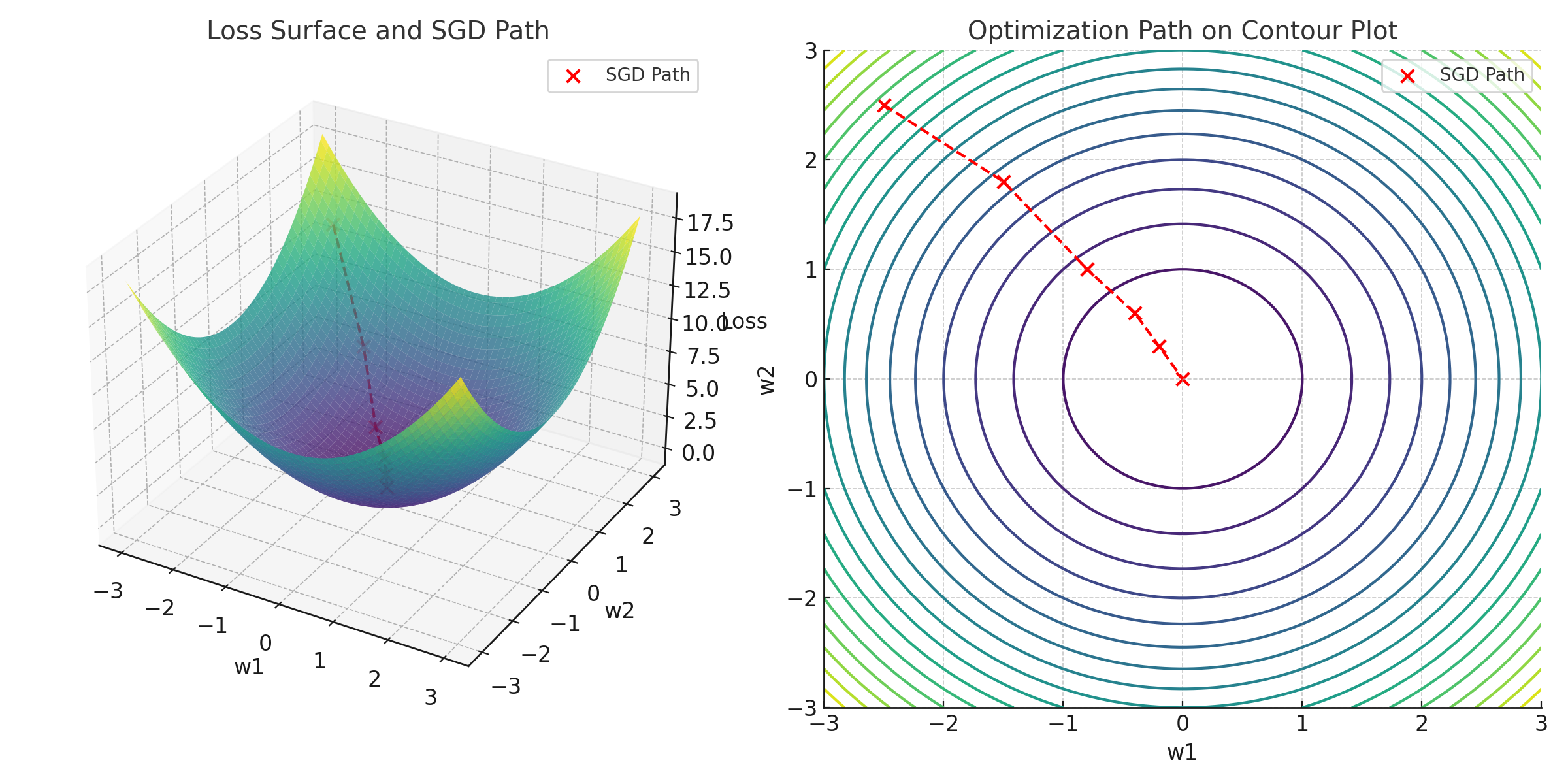
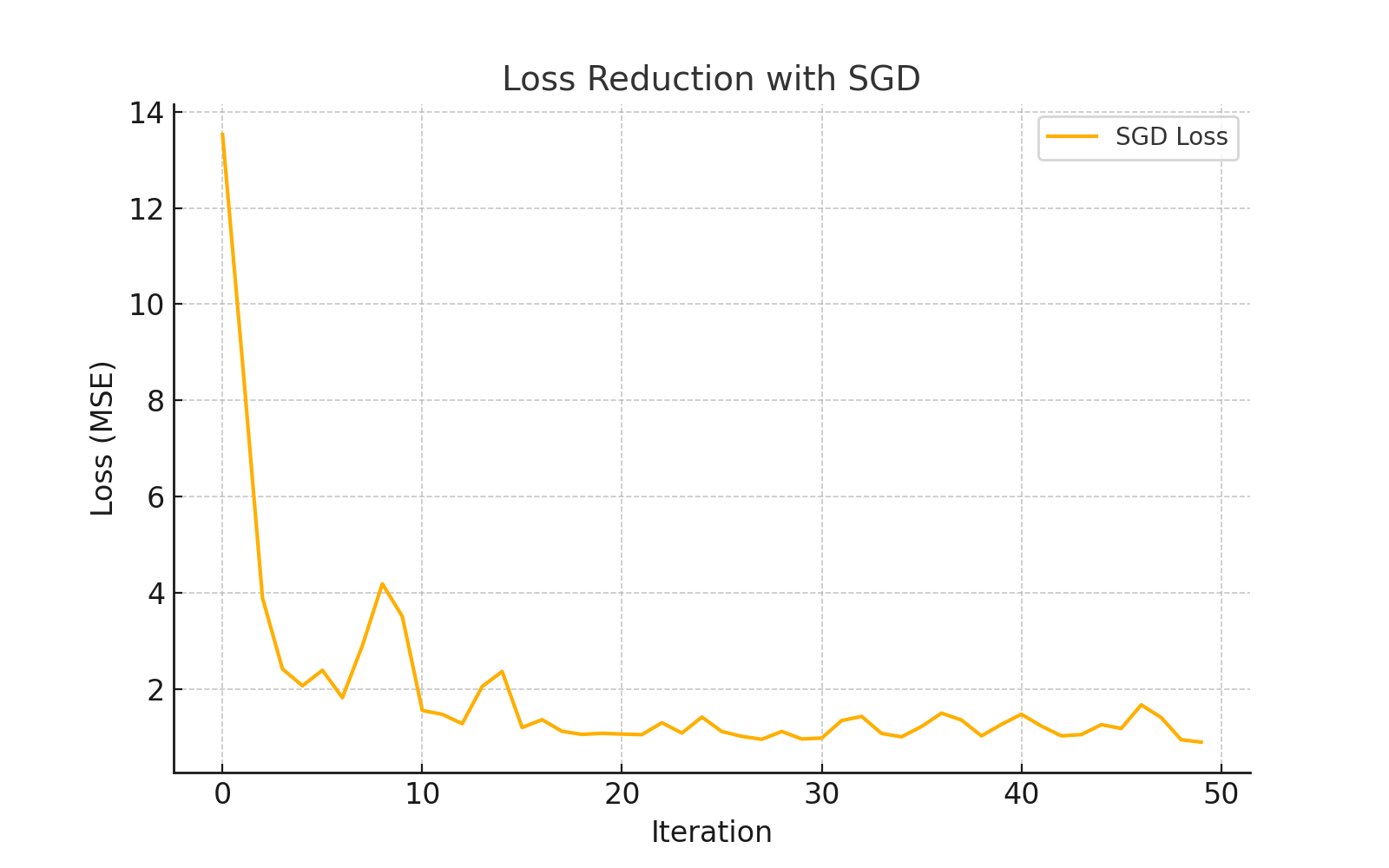
Visualization of SGD Optimization Path

The charts below illustrate how SGD iteratively reduces the loss and navigates the optimization landscape:

Saddle Point Challenges in Optimization

Non-convex loss surfaces often have saddle points where gradients vanish, making it difficult for SGD to progress. Adaptive optimizers like Adam can escape these regions more effectively. The chart below illustrates a simple loss surface with a saddle point:

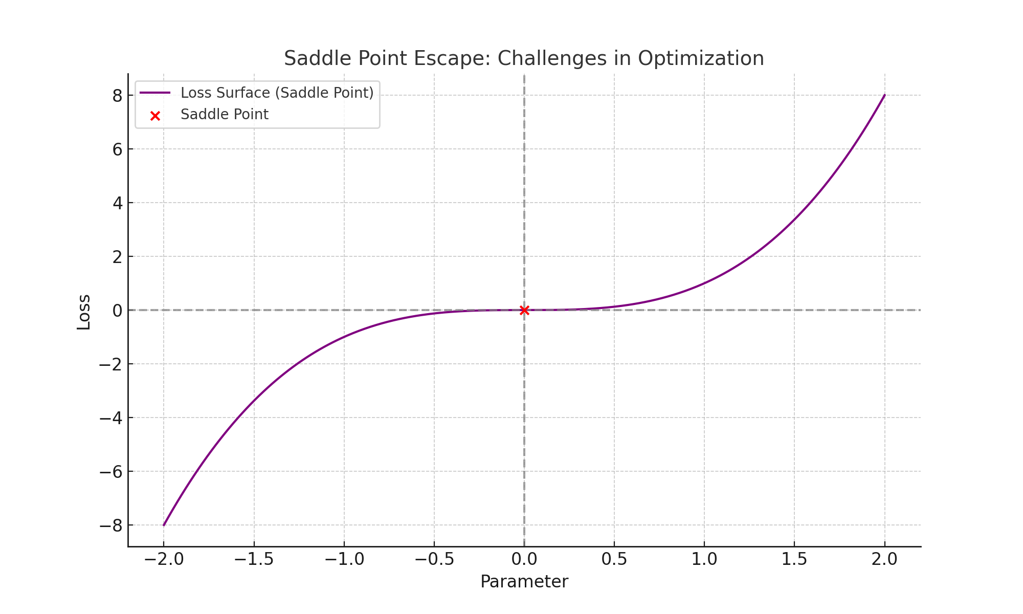
SGD may stagnate at the saddle point (red marker), while adaptive optimizers use their variance reduction properties to escape efficiently.

Challenges in Non-Convex Optimization

Non-convex loss surfaces, common in deep learning, introduce challenges like saddle points and local minima. Optimizers like SGD with Momentum and Adam are designed to handle these challenges effectively. The 3D plot below illustrates a non-convex loss surface:

Momentum in SGD

Momentum enhances Stochastic Gradient Descent (SGD) by accumulating a velocity term, which combines past gradients for smoother updates and faster convergence. The update rule is given by:

vt+1 = βvt + η∇f(wt),
wt+1 = wt - vt+1

Here:

• v_t: Velocity term, which accumulates past gradients.
• β: Momentum coefficient, determining the influence of past gradients.
• η: Learning rate, controlling step size.

How Momentum Works: Step-by-Step

1. Initial Step: Both SGD and Momentum take the first step based on the gradient at the starting point.
2. Accumulation of Velocity: Momentum combines past gradients using β for smoother updates.
3. Reduction in Oscillations: This reduces zig-zagging in noisy gradients, allowing faster convergence.
4. Convergence: Momentum uses its accumulated velocity to efficiently reach the true minimum.

Visual Explanation

The following visuals illustrate Momentum's advantages:

Path to Convergence: Momentum's trajectory (red) converges faster and more smoothly than plain SGD (blue):

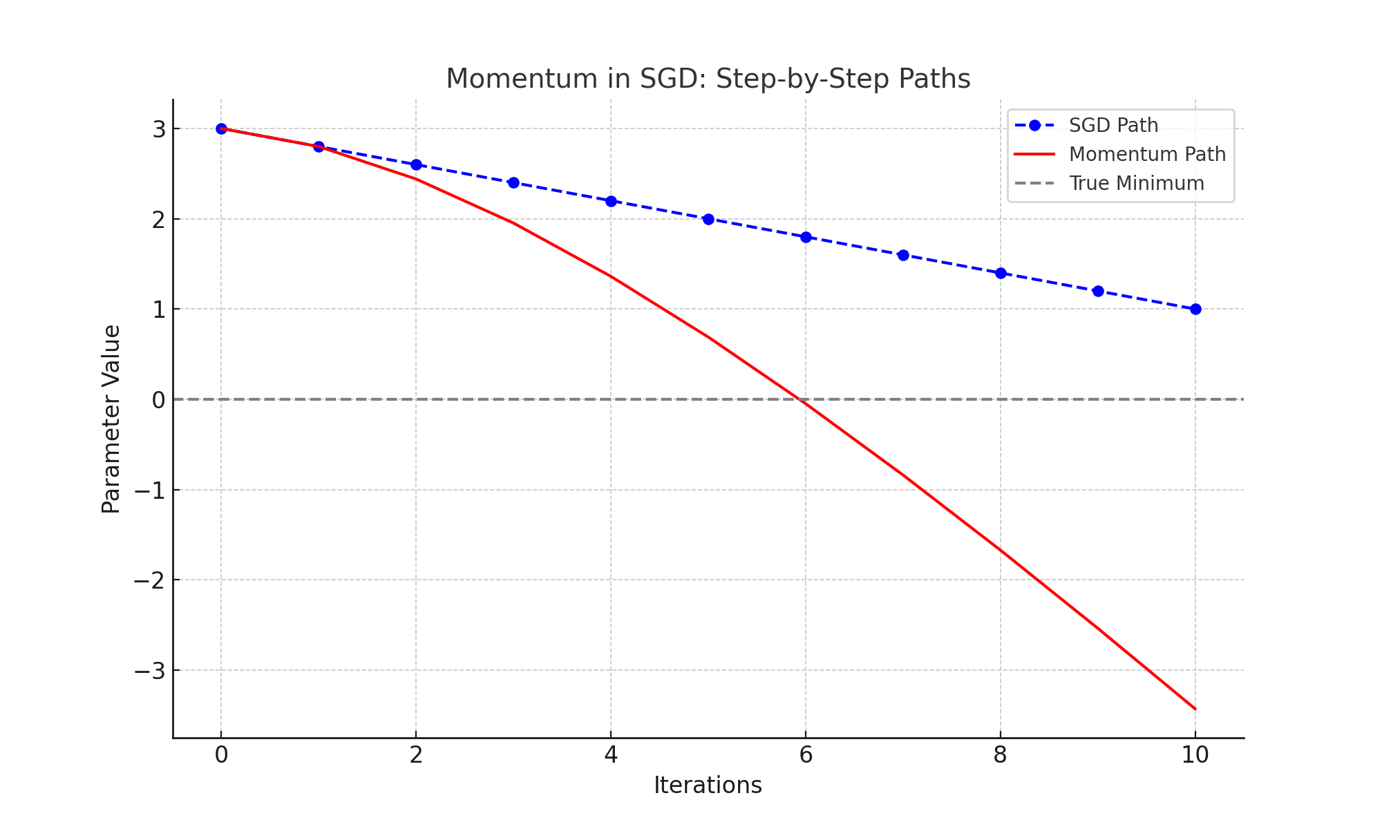
What Does "Parameter Value" Represent?

The parameter value in the graphs represents the optimization variable (e.g., w) that the algorithm adjusts to minimize the loss function. Here's what it signifies:

• Initial Value: Both SGD and Momentum start at an initial parameter value, which in this case is set to 3.
• Update Process:
  • SGD: Updates the parameter directly based on the gradient of the loss function.
  • Momentum: Incorporates past gradients to compute a smoother update via a velocity term.
• Convergence: The goal is to adjust the parameter iteratively, bringing it closer to the true minimum at 0.

This process is shown in the graphs, where the parameter value decreases over iterations until it converges to the optimal value, with Momentum demonstrating a faster and smoother trajectory compared to SGD.

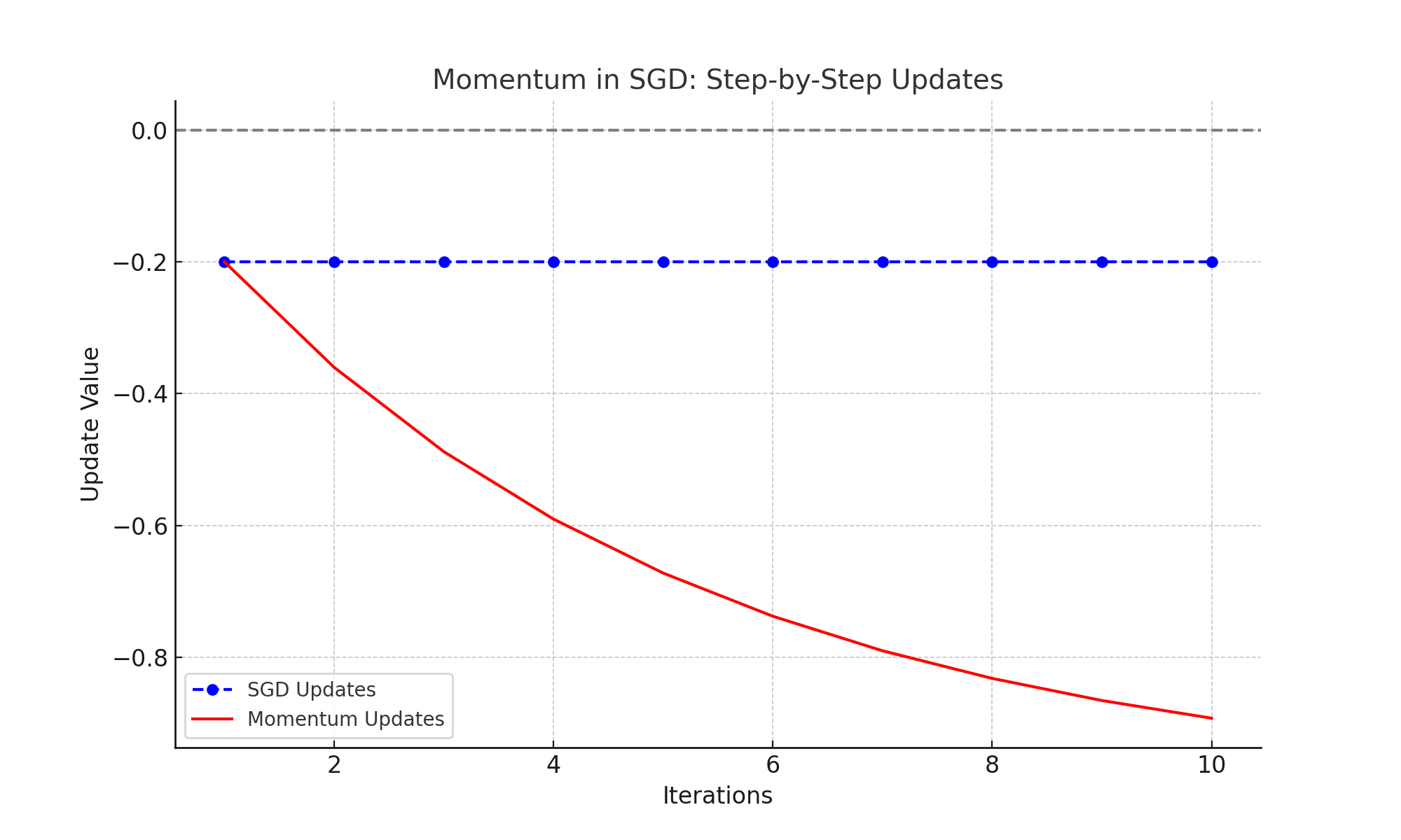
Update Dynamics: Momentum's updates start larger due to accumulated velocity but gradually decrease as it approaches the minimum:

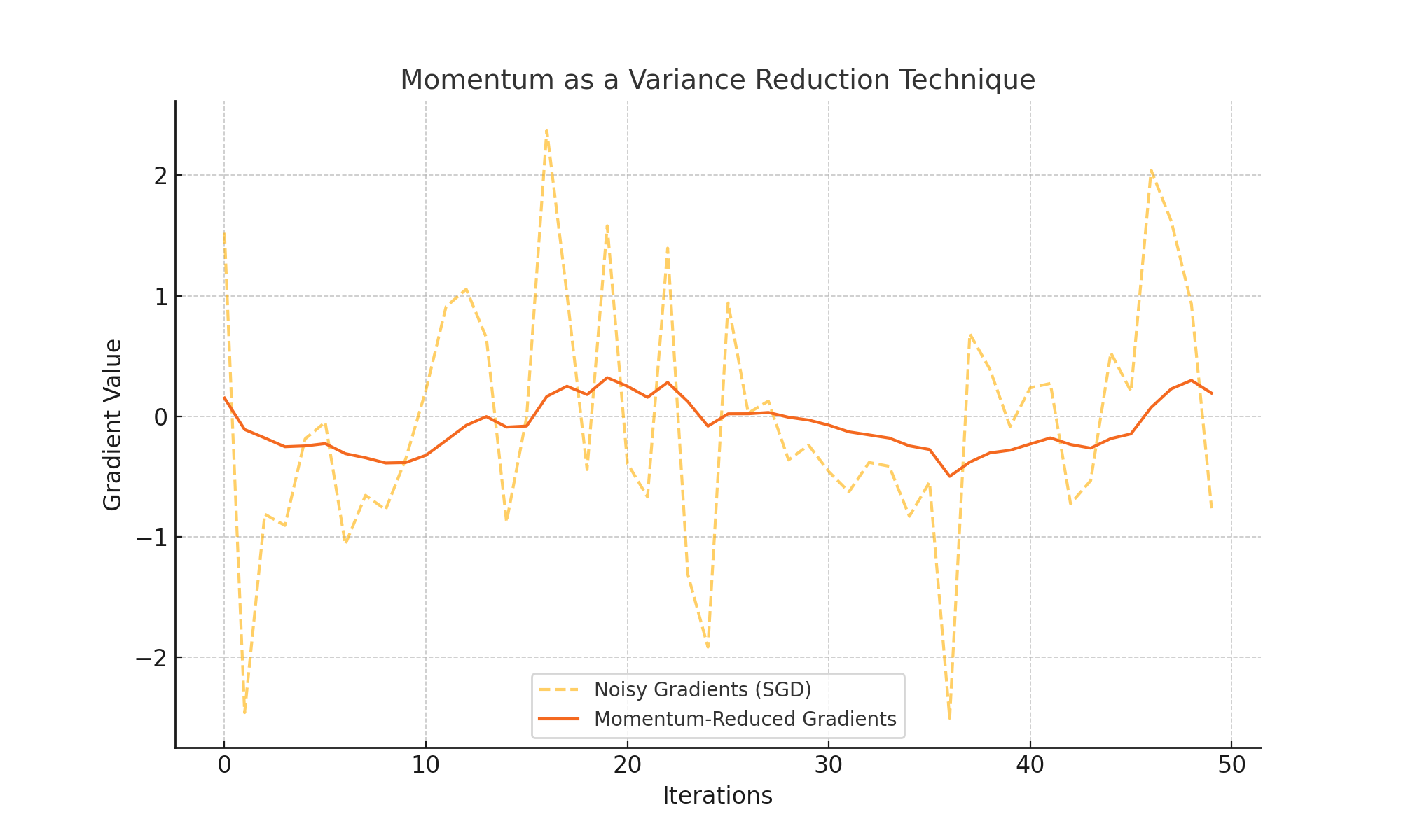
Momentum as a Variance Reduction Technique

Momentum not only accelerates convergence but also reduces the variance in gradient updates. This property makes optimization more stable, especially in noisy environments. The graph below shows how Momentum smooths noisy gradients:

Adam Optimizer: A Step Beyond

The Adam optimizer combines momentum and adaptive learning rates to enhance optimization:

mt = β1mt-1 + (1-β1)∇f(wt)
vt = β2vt-1 + (1-β2)(∇f(wt))2
wt+1 = wt - η mt / (√vt + ε)

Adam's adaptive learning rates and bias correction make it suitable for sparse gradients and complex models. However, in some scenarios, it may overfit compared to SGD with momentum.

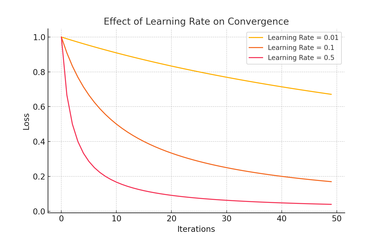
Learning Rate Tuning

The learning rate (η) is a crucial hyperparameter in SGD. A well-tuned learning rate ensures fast convergence without overshooting:

Challenges in SGD

While Stochastic Gradient Descent (SGD) is a cornerstone of optimization, it faces a few key challenges:

• Non-convex loss surfaces: Optimization can struggle with saddle points and local minima, slowing convergence.
• Gradient variance: High variance in gradient estimates can lead to unstable or noisy updates.
• Learning rate tuning: Finding the right learning rate is crucial for balancing speed and stability in optimization.

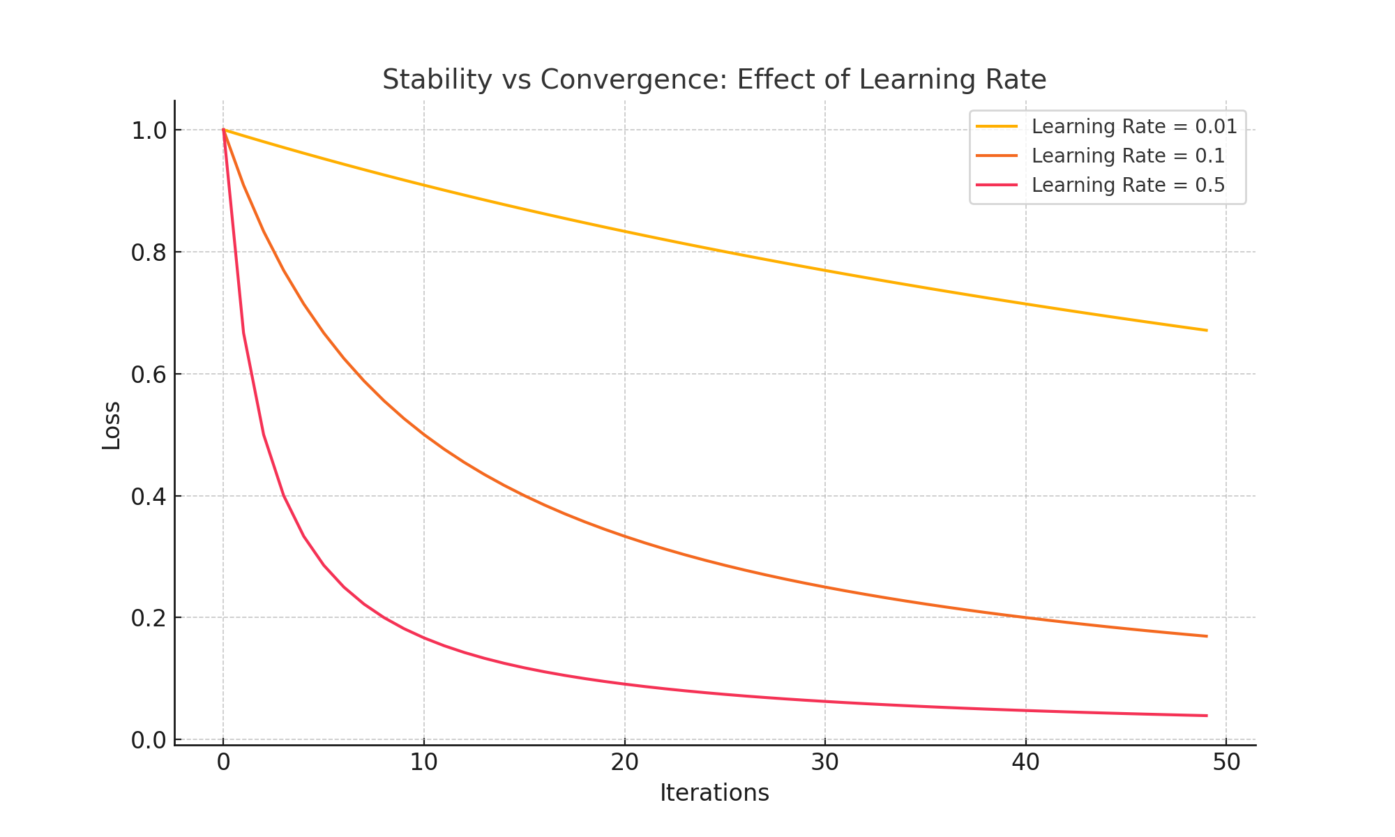
Balancing Stability and Convergence in SGD

Choosing the right learning rate is critical in SGD. A low learning rate ensures stability but slows convergence, while a high learning rate speeds up convergence but risks overshooting the minimum. The chart below illustrates this trade-off:

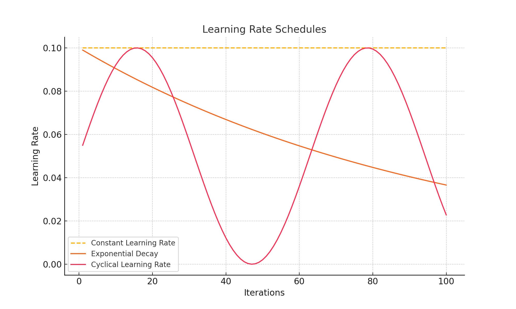
Learning Rate Schedules

Learning rate schedules control how the step size changes during optimization. Here are three common approaches:

• Constant: The learning rate remains fixed throughout training.
• Exponential Decay: The learning rate decreases gradually over time.
• Cyclical: The learning rate oscillates between a minimum and maximum value.

The chart below illustrates these schedules:

Advanced Learning Rate Strategies

Cosine annealing is an advanced learning rate strategy that periodically reduces and resets the learning rate, helping the optimizer explore the loss surface more effectively. The chart below shows how the learning rate evolves:

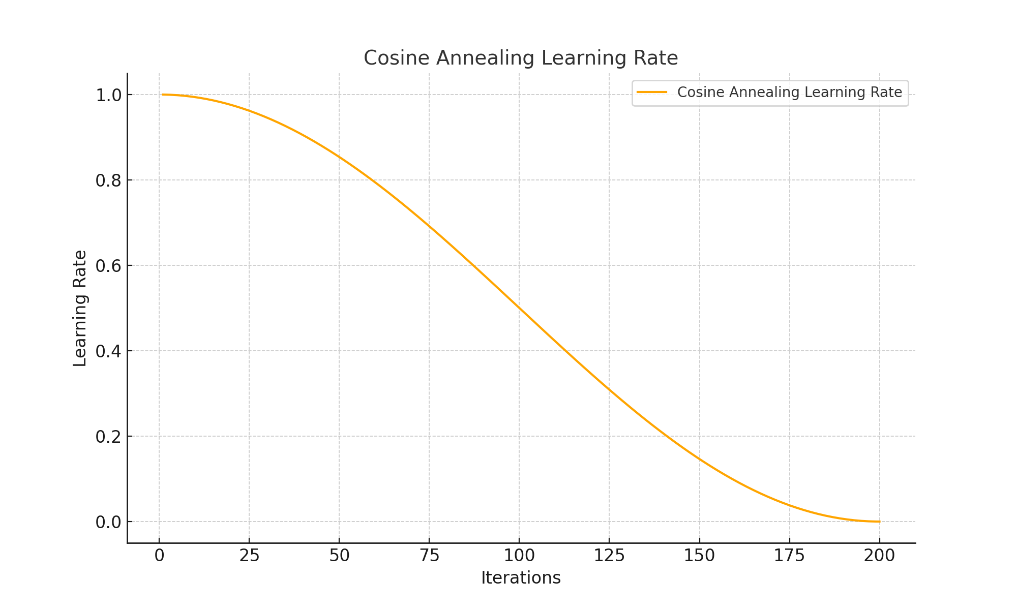
This approach is particularly useful in tasks where the optimization landscape has multiple local minima or sharp valleys.

Scaling SGD for Distributed Training

Distributed SGD enables large-scale training by dividing the workload across multiple machines or devices. Each worker computes gradients on a subset of data and contributes to the global model update.

Workflow

1. Gradient Calculation: Each worker computes its local gradient:
   gk = (1 / |Dk|) Σ ∇f(x; w)
2. Aggregation: Gradients are aggregated across workers:
   g = (1 / N) Σ gk
3. Parameter Update: The global model is updated:
   wt+1 = wt - η g
4. Global Model Distribution: The updated model is sent back to all workers.

Synchronous vs Asynchronous SGD

• Synchronous SGD: Workers compute and synchronize gradients simultaneously, ensuring consistency but slowing progress due to stragglers.
• Asynchronous SGD: Workers compute and send gradients independently, allowing faster updates but introducing potential staleness.

Challenges

• Communication Bottlenecks: Gradient transmission can overwhelm bandwidth. Solutions include gradient compression and reduced communication frequency.
• Straggler Effect: Slow workers delay synchronous SGD. Asynchronous methods mitigate this issue.
• Non-IID Data: Variations in data distribution can lead to biased gradients. Solutions include regularization during aggregation.

Improvements

• Gradient Compression: Compress gradients before transmission to save bandwidth:
  g̃k = Compress(gk)
• Decentralized SGD: Workers communicate directly without relying on a central server, enhancing robustness:
  wt+1k = wtk - η Σj ∇fj(wt)

Federated Learning with Distributed SGD

Federated Learning allows decentralized devices (e.g., smartphones, IoT devices) to collaboratively train machine learning models without sharing raw data, ensuring privacy and reducing communication overhead.

How It Works

1. Local Training: Each device computes its local gradient based on its dataset:
   wit+1 = wit - η ∇fi(wit)
2. Aggregation: The server aggregates these updates into a global model:
   wt+1 = Σ (|Di| / Σ |Dj|) wit+1
3. Global Model Distribution: The updated model is sent back to devices for further training.

Advantages

• Privacy: No raw data leaves the device; only gradients or model updates are shared.
• Scalability: Supports training across millions of devices.
• Personalization: Local models can be fine-tuned for specific devices after aggregation.

Challenges

• Non-IID Data: Data across devices may not follow the same distribution, leading to biased gradients.
• Communication Overhead: Frequent updates can strain bandwidth.
• Device Heterogeneity: Differences in computational power and data availability can cause delays.

Improvements: Federated Averaging (FedAvg)

To reduce communication, devices train locally for several epochs and send averaged updates:
wit+E = wit - η Σe=1E ∇fi(wit+e)

Applications and Real-World Use Cases

SGD is integral to many machine learning workflows, powering applications such as:

• Deep neural networks: Efficiently trains large models like CNNs and RNNs for tasks such as image recognition and natural language processing.
• Logistic regression: Plays a vital role in solving binary classification problems across industries.
• Reinforcement learning: Optimizes sequential decision-making tasks in robotics, gaming, and AI systems.

Case Study: Training ResNet with SGD and Momentum

ResNet, a deep convolutional neural network, highlights the advantages of Momentum in training large models. The chart below compares training loss across epochs for SGD and Momentum:

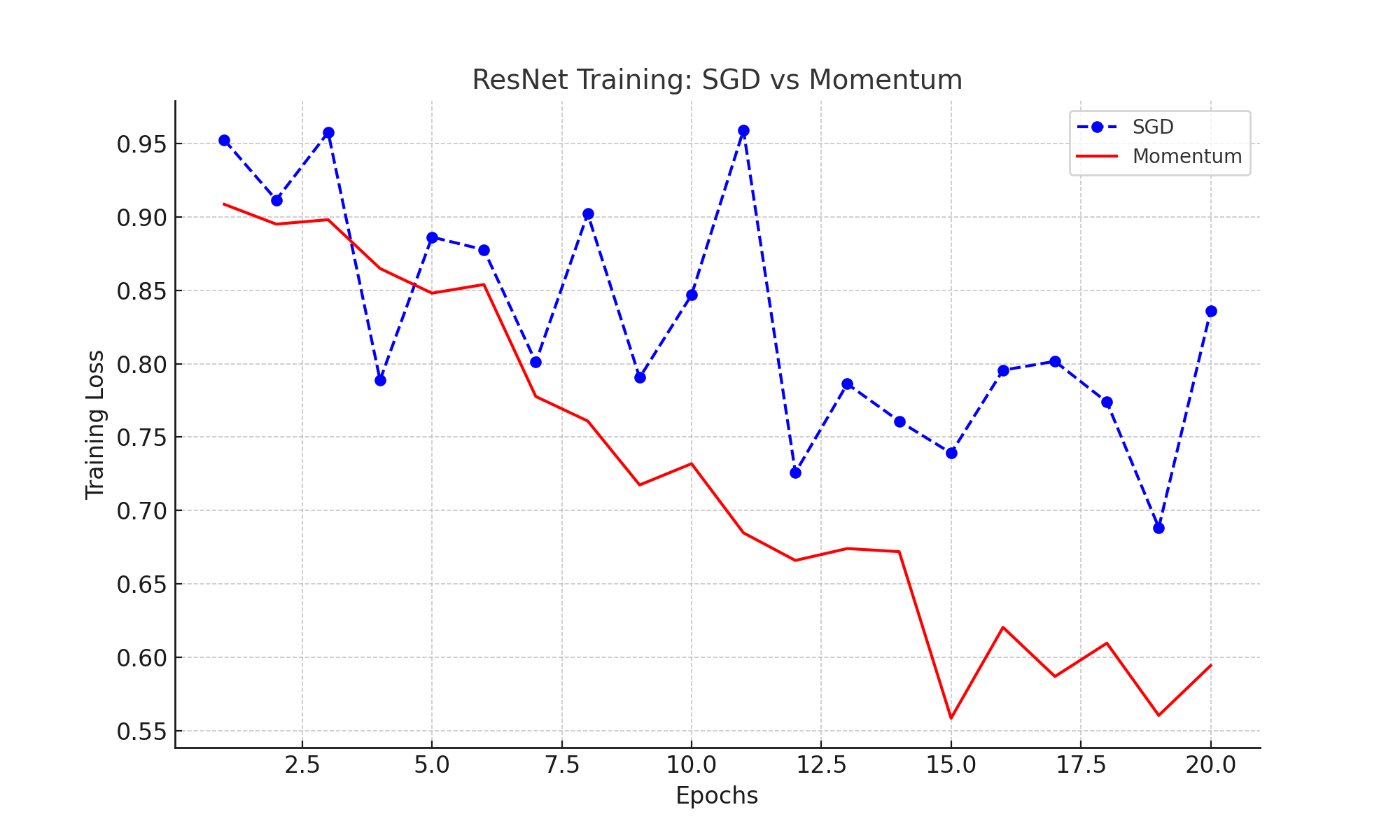
Insights:

• SGD: Slower convergence and higher oscillations in loss values.
• Momentum: Reduces oscillations, leading to faster and more stable convergence.

Adaptive Optimization Techniques

While SGD is a powerful optimizer, adaptive methods like Adam and RMSProp provide faster convergence in many scenarios by adjusting learning rates dynamically. The chart below compares their performance:

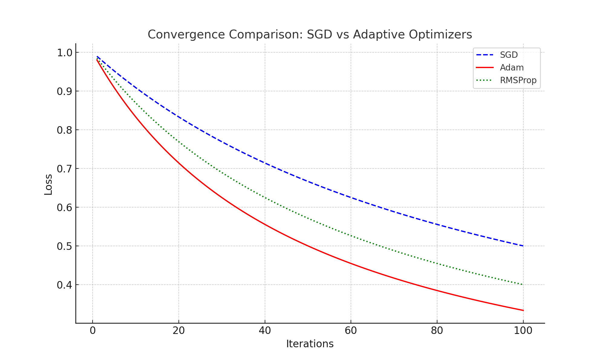
Key Observations:

• SGD: Slower convergence but better generalization in some cases.
• Adam: Faster convergence due to momentum and adaptive learning rates.
• RMSProp: Similar to Adam but simpler, effective for certain tasks.

Comparison Between Adam and SGD

Feature	SGD	Adam
Learning Rate	Fixed or manually adjusted	Adaptive and parameter-specific
Momentum	Optional	Built-in
Convergence Speed	Slower	Faster
Handling Sparse Gradients	Poor	Excellent
Generalization	Often better	May overfit in some scenarios

Optimizer Summary

Optimizer	Key Features	Benefits	Challenges
SGD	Basic stochastic updates	Simple, scales well	Slow convergence
Momentum	Incorporates velocity	Smoother updates	Requires tuning β
Adam	Adaptive learning rates	Fast convergence	May overfit
RMSProp	Adaptive step size	Handles non-stationary objectives	More hyperparameter tuning

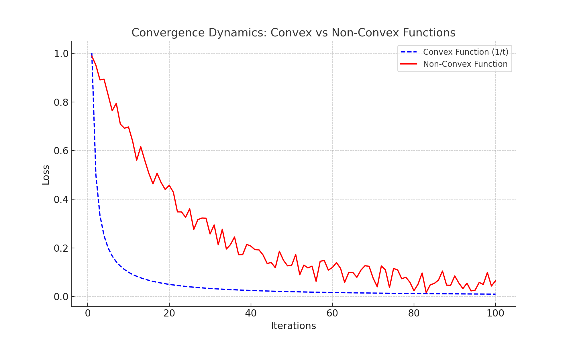
Convergence Dynamics: Convex vs Non-Convex Functions

The convergence of SGD varies based on the function landscape. For convex functions, the loss decreases at a rate of 1/t, while non-convex landscapes introduce variability due to local minima and saddle points. The plot below illustrates these dynamics:

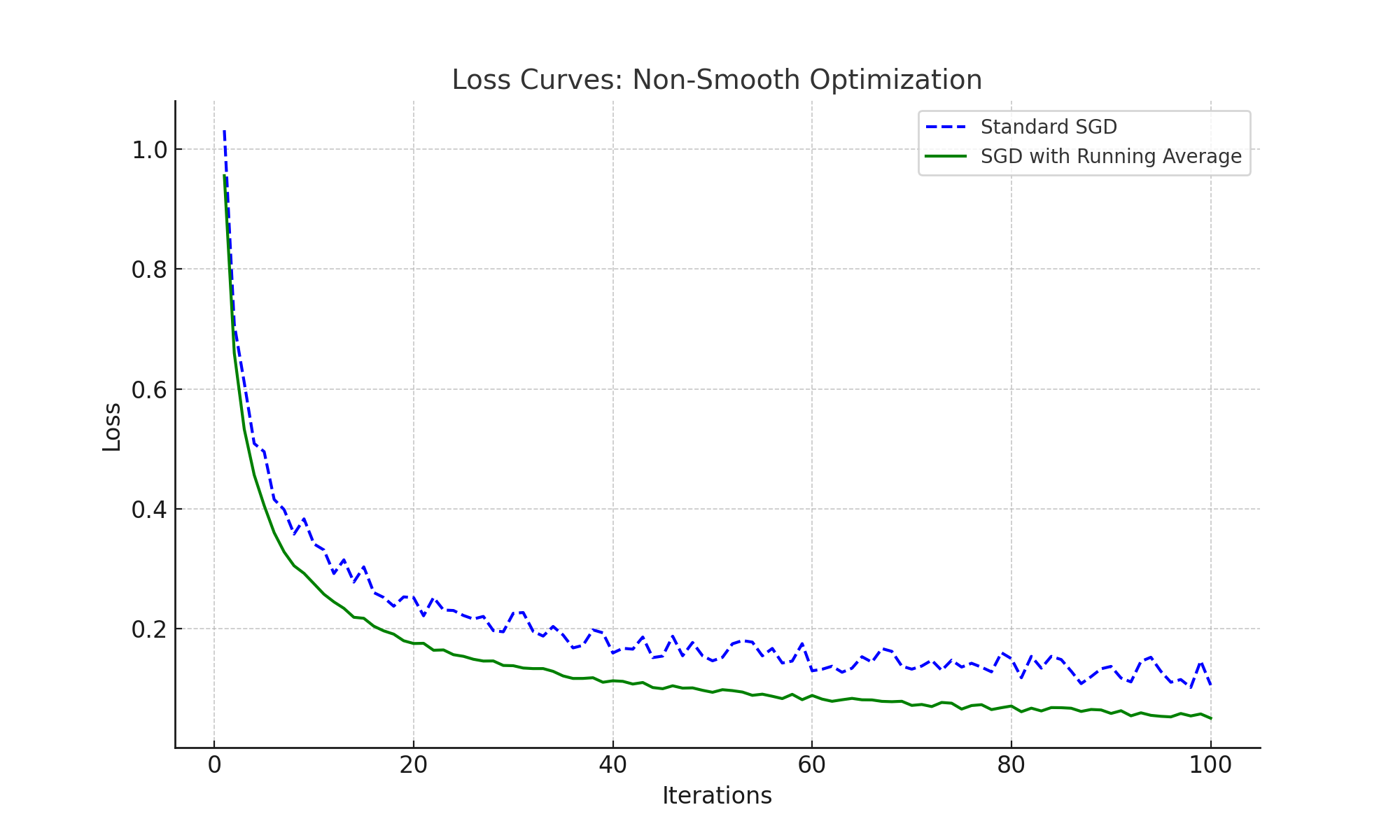
Loss Curves for Non-Smooth Optimization

Non-smooth optimization problems present challenges for standard SGD due to irregular gradients. Using running averages helps stabilize updates, as seen in the loss curves below:

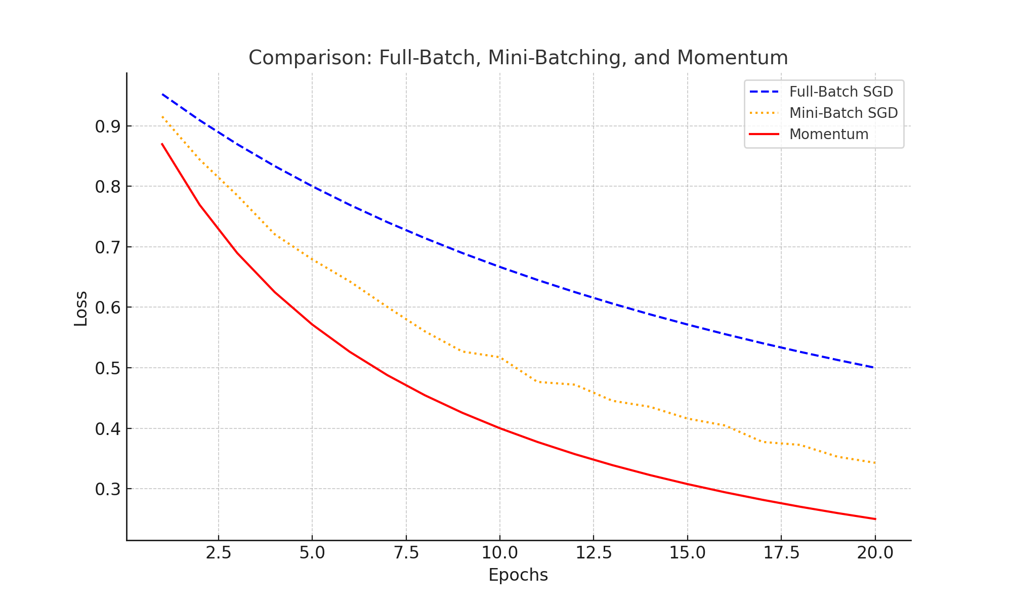
Comparison: Full-Batch, Mini-Batching, and Momentum

Mini-batching reduces gradient variance, and momentum smooths updates, accelerating convergence compared to full-batch SGD. The plot below highlights their effects on loss reduction:

Optimization Paths under SDE Noise Levels

Viewing SGD as a discretization of a stochastic differential equation (SDE) reveals how noise influences optimization paths. The plot below shows paths under low and high noise levels:

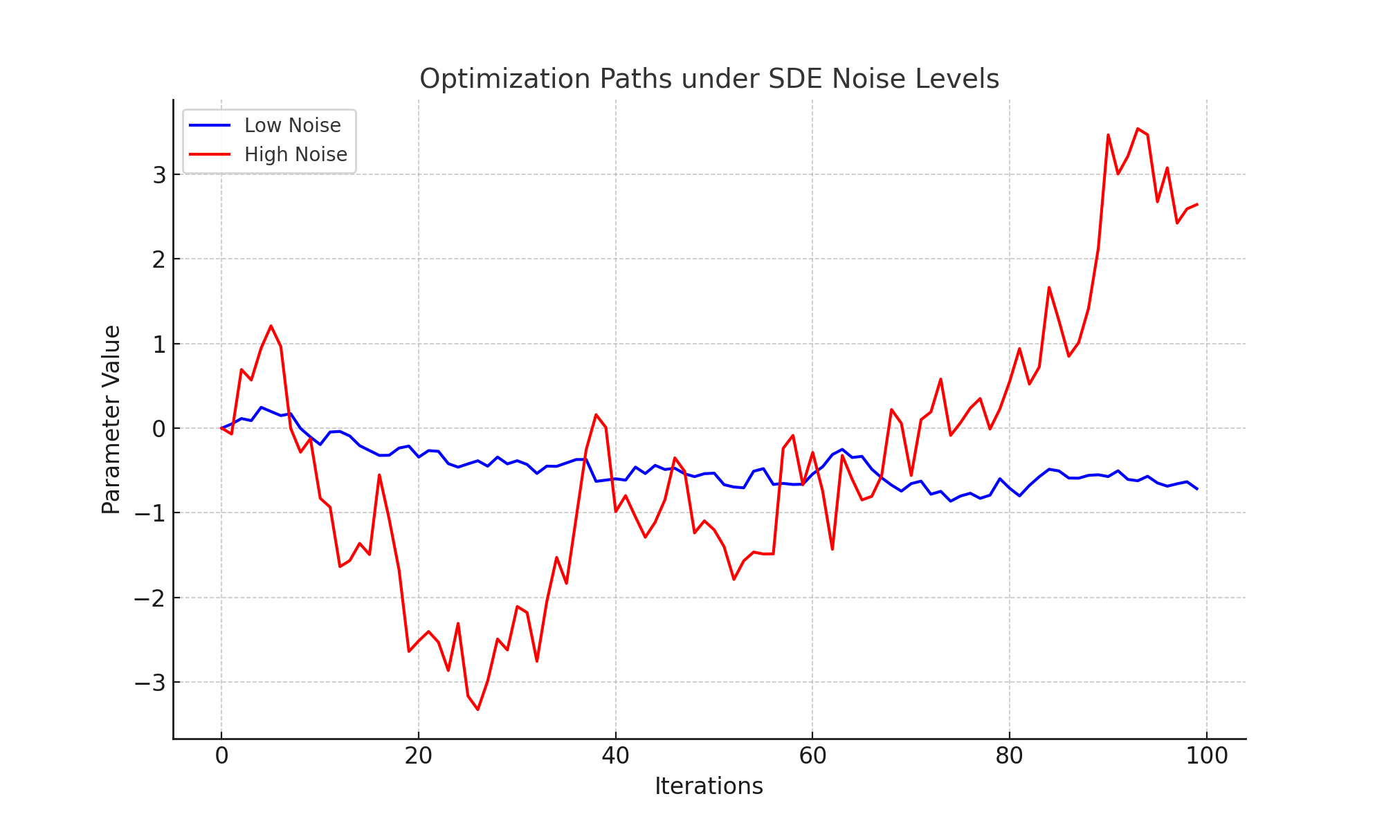
High noise levels encourage exploration but reduce stability, while low noise levels favor stability but may lead to suboptimal convergence.

High-Dimensional Non-Convex Landscapes

High-dimensional, non-convex optimization landscapes present significant challenges for SGD. The 3D plot below illustrates a complex surface with multiple local minima and saddle points:

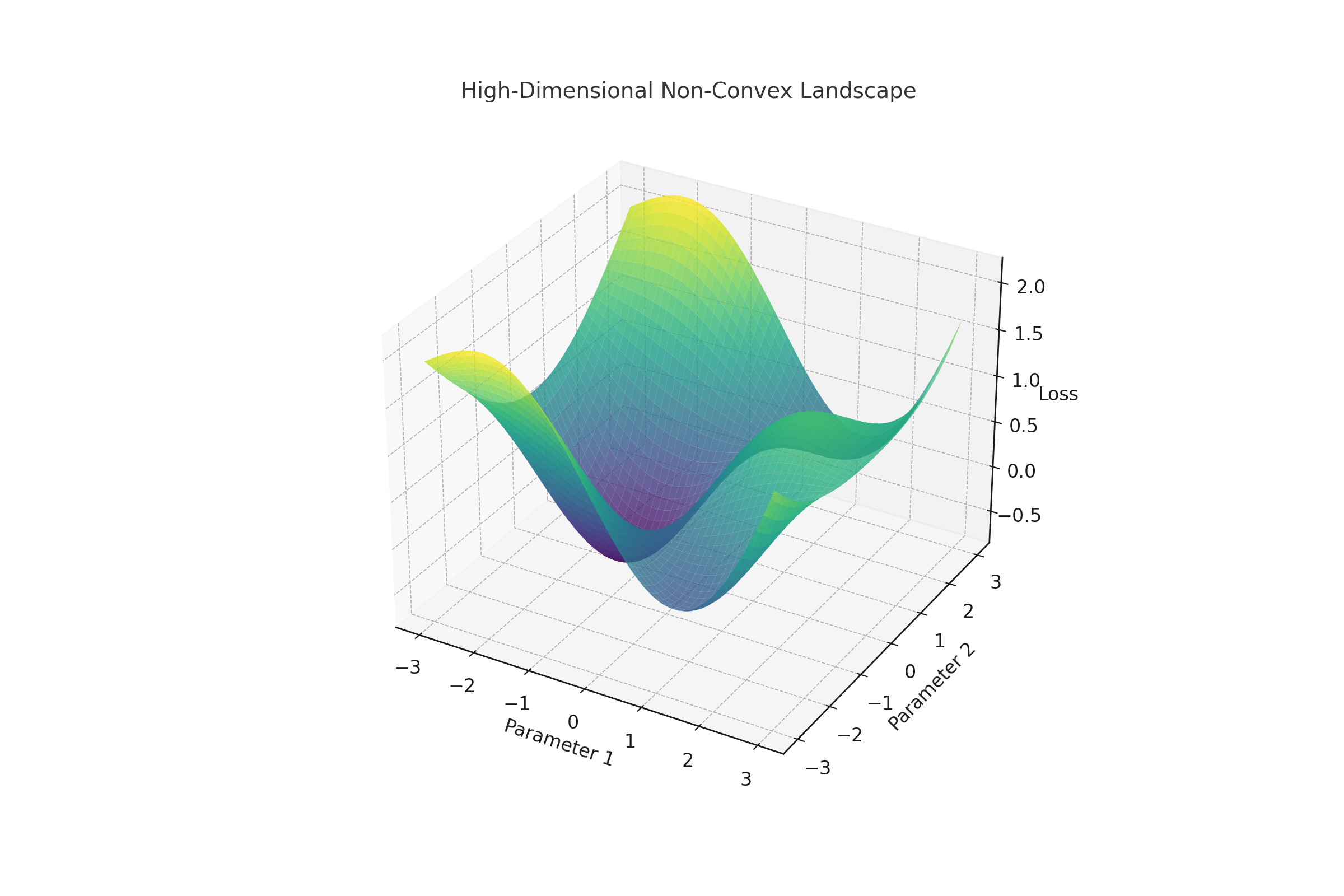
SGD's stochasticity enables efficient navigation of such landscapes, often outperforming deterministic gradient descent in these scenarios.

SGD's Role in Deep Learning

Stochastic Gradient Descent (SGD) is at the heart of deep learning optimization, enabling the training of models with millions or billions of parameters. Its scalability, stochastic updates, and effectiveness in exploring complex loss landscapes make it essential for deep learning tasks.

Why is SGD Important?

• Handles High-Dimensional Parameter Spaces: Essential for optimizing deep models with billions of parameters.
• Stochastic Updates: Reduces computational overhead, making training feasible on massive datasets.
• Explores Non-Convex Loss Surfaces: Helps escape saddle points and sharp minima, improving convergence.

The Evolution of Stochastic Gradient Descent (SGD)

Stochastic Gradient Descent (SGD) has a rich history spanning several decades, evolving from a simple optimization technique to a cornerstone of modern machine learning. Here's a timeline of key milestones:

1950s: The Birth of Gradient Descent

The roots of SGD trace back to classical gradient descent, introduced as a method to solve optimization problems in numerical analysis. The method relied on iterative updates to minimize functions.

1960s: Robbins-Monro Algorithm

In 1951, Herbert Robbins and Sutton Monro proposed the stochastic approximation method, laying the foundation for SGD. Their work formalized the use of noisy gradients to approximate true gradients, making the method computationally efficient.

1980s: Neural Networks and Backpropagation

SGD gained prominence in the 1980s with the rise of artificial neural networks. Backpropagation, introduced by Rumelhart, Hinton, and Williams in 1986, relied heavily on SGD for updating model weights.

1990s: Mini-Batch SGD

The concept of mini-batch SGD emerged, balancing the computational efficiency of SGD with the stability of full-batch gradient descent. This advancement made SGD more practical for large datasets.

2010s: Deep Learning Renaissance

• 2012: SGD played a critical role in training AlexNet, the model that won the ImageNet competition and sparked the deep learning revolution.
• 2014: Momentum and adaptive methods like Adam were introduced, improving SGD's convergence in non-convex problems.
• 2017: Transformers and attention mechanisms emerged, with SGD variants powering their optimization.

2020s: Scaling SGD for Large Models

With models like GPT-3 and GPT-4 containing billions of parameters, SGD has scaled through techniques like distributed training, gradient accumulation, and federated learning. Novel optimizers such as Lion and QH-Momentum further enhanced its capabilities.

2024: Recent Advances

Research in 2024 has focused on enhancing SGD's theoretical foundations, developing adaptive frameworks for non-smooth optimization, and leveraging SGD in specialized domains like reinforcement learning and federated systems.

Variants of SGD in Deep Learning

• SGD with Momentum: Smooths updates and accelerates convergence, commonly used in CNNs like ResNet.
• Adam Optimizer: Combines momentum with adaptive learning rates, effective for sparse gradients in transformers.
• RMSProp: Dynamically scales learning rates, useful in RNNs for sequential data.

Equations

SGD's core update rule and its variants:

• SGD Update: wt+1 = wt - η ∇L(wt)
• Momentum: vt+1 = βvt + (1-β) ∇L(wt), wt+1 = wt - ηvt+1
• Learning Rate Schedules:
  • Exponential Decay: ηt = η0 ⋅ e-λt
  • Cosine Annealing: ηt = ηmin + (ηmax - ηmin) / 2 ⋅ (1 + cos(πt/T))

SGD in Architectures

• CNNs: Trains models like ResNet for image tasks using momentum and weight decay.
• RNNs: Leverages RMSProp for handling sequential dependencies.
• Transformers: Adam and distributed SGD power massive models like GPT and BERT.

SGD in Transformer Architectures like GPT

Stochastic Gradient Descent (SGD) and its variants, particularly Adam, are pivotal in training transformer-based architectures like GPT. These models have billions of parameters, making scalability, sparse gradients, and efficient optimization critical for success.

Why SGD is Essential

• Handles High-Dimensional Parameter Spaces: Optimizes billions of parameters efficiently.
• Sparse Gradients: Adapts to the sparse updates common in attention mechanisms.
• Non-Convex Optimization: Stochasticity aids in escaping saddle points and exploring complex landscapes.

Challenges in Transformer Training

• Exploding Gradients: Managed using gradient clipping:
  g = g / max(1, ||g|| / c)
• Learning Rate Scheduling: Warm-up and decay schedules stabilize training:
  ηt = ηmax ⋅ min(t / Twarmup, Tdecay / t)
• Distributed Training: Gradient accumulation and federated averaging ensure scalability.

Exploding Gradients

Exploding gradients occur due to large gradient magnitudes in deep transformers, particularly when processing long sequences. Gradient clipping mitigates this by capping gradient norms at a specified threshold:

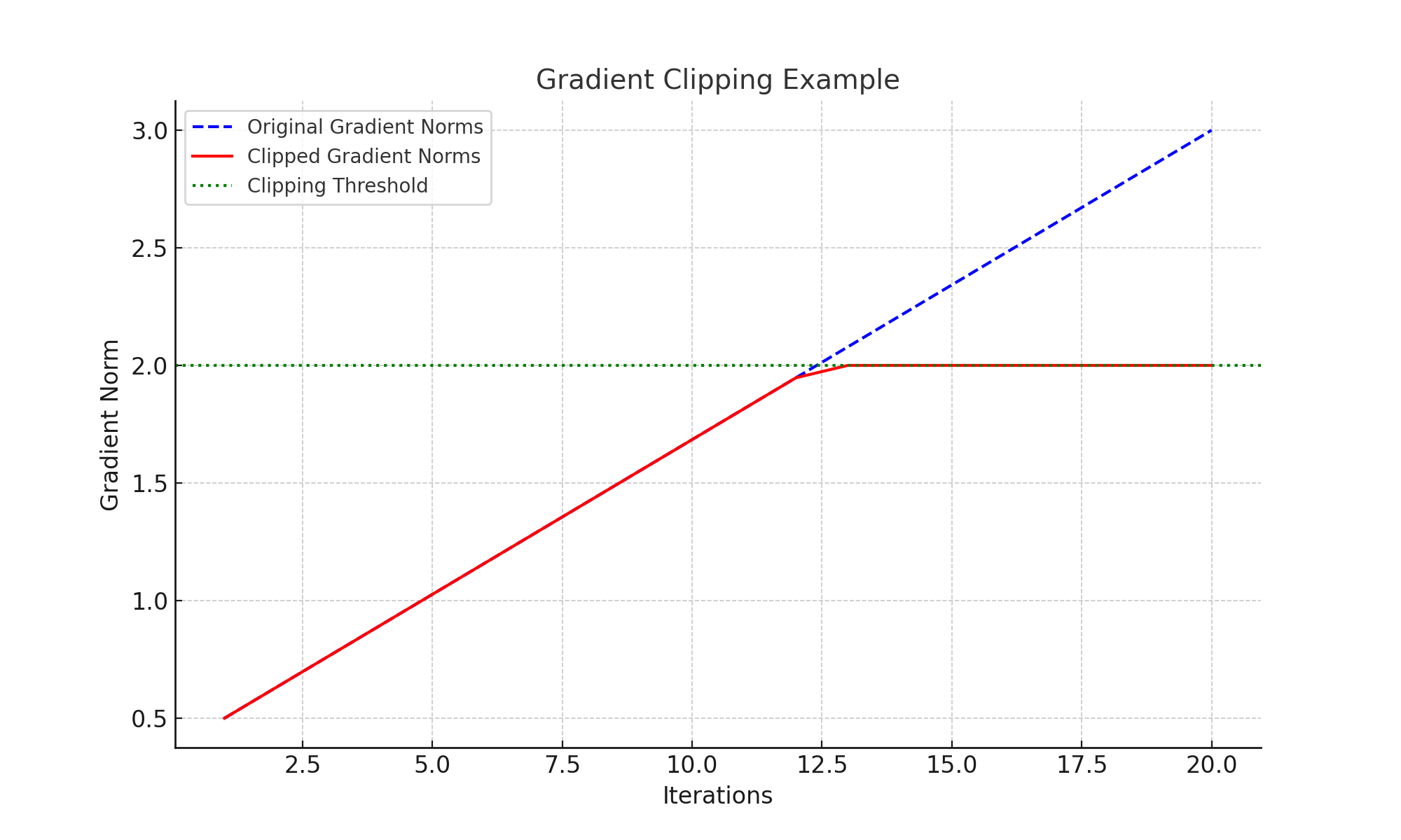
Clipping ensures stability without drastically altering the optimization dynamics, making it essential for training large models.

Key Contributions

• Layer-Wise Adaptive Rate Scaling (LARS): Adjusts learning rates for each layer based on gradient magnitudes.
• Gradient Accumulation: Reduces memory usage while simulating large batch sizes.
• Pre-training and Fine-Tuning: Optimizes both massive corpora pre-training and task-specific fine-tuning.

Equations for Transformer Training

• Parameter Update with Weight Decay: wt+1 = wt - η (∇L(wt) + λwt)
• Gradient Clipping: g = g / max(1, ||g|| / c)
• Learning Rate Schedules:
  • Warm-up: ηt = ηmax ⋅ t / Twarmup
  • Decay: ηt = ηmax ⋅ Tdecay / t

Learning Rate Scheduling

Training transformers involves careful learning rate schedules to stabilize optimization. The warm-up phase prevents large initial updates, while decay gradually reduces the learning rate to refine the optimization:

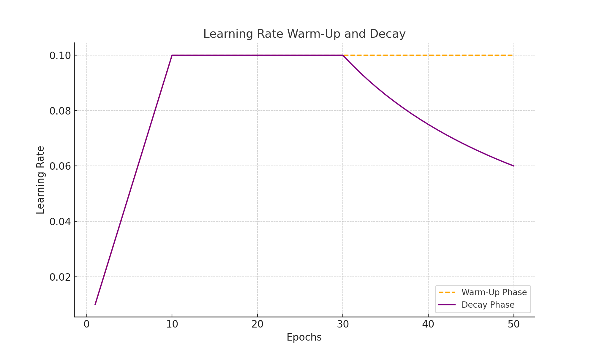
This approach helps achieve a balance between fast convergence during initial training and stability in later stages.

Conclusion

Stochastic Gradient Descent is a versatile and efficient optimization method that forms the backbone of many machine learning algorithms. Its variants, such as SGD with momentum and Adam, offer additional flexibility and performance improvements for specific use cases.

Key Takeaways

• SGD: Efficient for large datasets but sensitive to learning rate and gradient variance.
• Momentum: Acts as a variance reduction mechanism, smoothing updates and accelerating convergence.
• Adam: Combines momentum with adaptive learning rates, excelling in sparse and noisy environments.
• Applications: Widely used in deep learning, logistic regression, and reinforcement learning tasks.

Future Directions

Exploration of hybrid optimizers that combine the strengths of different methods is an ongoing research area. Techniques like cyclical learning rates and advanced variance reduction methods are also promising avenues for improving optimization efficiency.

Understanding the nuances of optimization algorithms like SGD, Momentum, and Adam empowers practitioners to make informed decisions for training robust and efficient machine learning models.